FETISH: An Introduction

Here, I will give an explanation of what the FETISH Rust library crate does by utilizing two other tools that I’ve developed as part of the ecosystem: FETISH-CONSTRUCTOR and FETISH-INSPECTOR. While I have posted previously about FETISH, the existing links there are primarily for an academic audience. This guide, on the other hand, is much more experiential, so feel free to jump in and follow along!

Introduction

FETISH, or “Functional Embedding of Terms In a Spatial Hierarchy”, is a mechanism for statistically modeling the behavior of terms in a small functional language in such a way that we may obtain vector embeddings for such terms, which in turn enables the use of classic machine learning algorithms in the rather complex domain of programming, very similar to how embeddings enable natural language processing through ML.

Below is a brief, guided tour of FETISH using extant open-source tooling, provided in Rust.

Setup

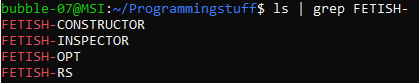
First, we’ll want to clone down the FETISH-RS, FETISH-CONSTRUCTOR and FETISH-INSPECTOR repositories into a common base directory that we’ll be able to easily reference later. In my case, I chose ~/Programmingstuff:

Then, using cargo, build FETISH-CONSTRUCTOR from inside that directory – this is needed to generate a dynamic library describing a way to generate an operating specification for the base language that our FETISH instance will operate on. This dynamic library, in turn, will later be loaded and utilized by FETISH-INSPECTOR, which is kind of like a REPL for FETISH.

Finally, you’ll want to create a new sample_context.json file which you’ll easily be able to reference later (In my case, I chose to put it in ~/Programmingstuff.) In general, depending on the FETISH dynamic library built, the format of this JSON file may be radically different from the sample below, which is a sample configuration for the dynamic library provided by FETISH-CONSTRUCTOR in particular.

{
    "cauchy_scaling" : 1.0,
    "fourier_coverage_multiplier" : 3,
    "fourier_importance" : 0.1,
    "quad_padding_multiplier" : 1,
    "quad_importance" : 0.1,
    "lin_importance" : 0.8,
    "dim" : 2,
    "dim_taper_start" : 4,
    "elaborator_prior_params" : {
        "error_covariance_prior_observations_per_dimension" : 10.0,
        "out_covariance_multiplier" : 2.0,
        "in_precision_multiplier" : 0.5
    },
    "term_prior_params" : {
        "error_covariance_prior_observations_per_dimension" : 10.0,
        "out_covariance_multiplier" : 2.0,
        "in_precision_multiplier" : 0.5
    }
}

Starting FETISH-INSPECTOR

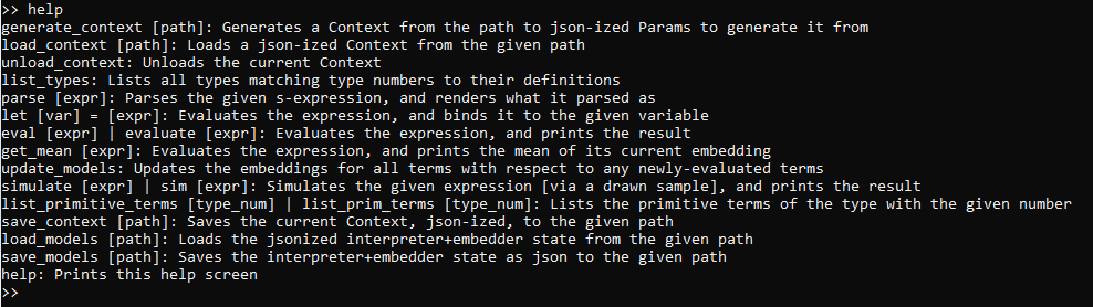
Inside of the FETISH-INSPECTOR directory, run cargo run [PATH_TO_FETISH_CONSTRUCTOR]/target/debug/libfetish_constructor.so. Once you do so, you will be presented with a >> prompt which comprises the prompt for the FETISH REPL. Within this prompt, several commands are available, and brief summaries of all of them may be provided by entering the help command, like so:

Generating a Context

Before performing most other actions described on the previous help screen, we’ll need to first generate a new “Context” from the dynamic library that we just passed in to FETISH-INSPECTOR upon start-up. Whereas the dynamic library we loaded provides a blueprint for how to construct base languages to use the inspector on, we need to supply a the .json parameters we specified earlier in order to actually construct one. To do so, we may execute the following command:

The command will take a few seconds to run as the specification for the base language is generated, but after it has finished, we’ll once again get the >> prompt for us to enter more commands.

#Listing Types and Primitive Terms

Now that we have a context, we can begin to inspect what was generated. To start with, since FETISH-based languages are all simply-typed, and have finitely many types, all of which are either vector types or function types between other types, we may obtain an exhaustive enumeration of all types using the list_types command:

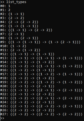
The way to interpret the output of the list_types command is that the enumeration for each particular type is listed to the left of the colon, and to the right of the colon is a visual rendering of what the type “is”. This format may seem confusing at first, but some worked examples should clear up any confusion:

• #0: 1: The type #0 is just a vector type with dimensionality 1.
• #1: 2: The type #1 is also just a vector type with dimensionality 2.
• #2: (1 -> 1): The type #2 is a function type with a 1-dimensional vector type [in our case, this must be #0] as its domain, and a 1-dimensional vector type [in our case, this must also be #0] as its codomain.
• #3: (2 -> 2): Just like the previous case, but instead the domain and codomain are both a 2-dimensional vector type [so in our case, these must both be #1]

• #4: (2 -> (2 -> 2)): This is a curried two-argument function on 2-dimensional vector types yielding another 2-dimensional vector type [all of which must be the type #1], or alternatively, we may view this as a function type whose domain is a 2-dimensional vector type #1 and whose codomain is the function type #3.

• … and so on

In the listing of types pictured, most of the types near the top of the list are inhabited by a wide variety of primitive terms, whereas types #12 and up by and by large are either inhabited by an instance of a primitive term for function composition, or are types which are not initially inhabited at all, but must exist to ensure closure under partial application of the composition primitive.

To view the primitive terms of each type, you may execute list_primitive_terms n to list all of the terms of the type numbered n. As we described in the previous paragraph, here are the results for both the initial segment of type numbers, and the segment for type numbers above 12:

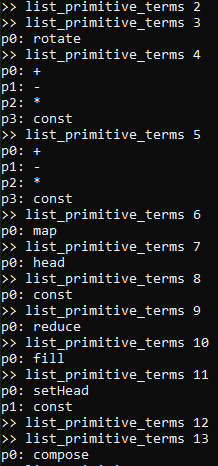
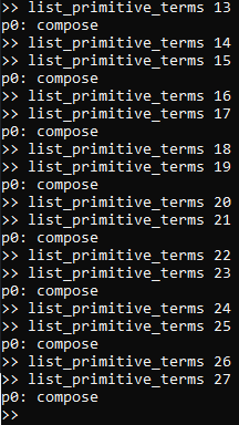
Cross-referencing the above results with the type enumeration results from the output of list_types, we can see, for instance:

• There is a primitive function which calls itself rotate and may be uniquely referred to as #3p0, with a domain and co-domain of two-dimensional vectors of type #1.
• There is a primitive function which calls itself + and may be uniquely referred to as #4p0, with a domain of two-dimensional vectors of type #1 and co-domain of #3.
• There is a primitive function which calls itself + and may be uniquely referred to as #5p0, with a domain of one-dimensional vectors of type #0 and co-domain of #2.
• … and so on.

Evaluating Term Applications

To try out the primitive function terms described above, we may use the eval command followed by a LISP-style S-expression for the term application which we wish to evaluate. For instance:

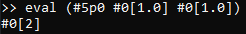
Here, we passed two vectors with the same value, #0[1.0] (a vector inhabitant of #0 with the particular vector value [1.0]) to the function term #5p0, which is a (curried) two-argument function which calls itself +. The result we got was #0[2], which is a vector inhabitant of #0 with the vector value [2]. In other words, we just evaluated 1 + 1, and got 2, as expected.

Given that the type signature of + as in #5p0 is curried as 1 -> (1 -> 1), we may be curious about the result of eval-ing a version of the above expression with only the first argument. The result is as follows:

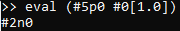
Every time we partially apply a primitive function term, we obtain a non-primitive function term, which is newly-allocated provided that we haven’t evaluated the same partial application before. Here, we obtained a new nonprimitive term n0 in the type #2, which based on the above discussion, we might be tempted to refer to informally as the “+1 function term”, or similar. However, from within expressions, the only way we know to refer to it at the moment is as its formal name, #2n0.

We can substantially improve this situation by introducing a let-binding for the name +1 to bind it to #2n0 as follows:

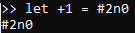
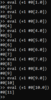
Once we have done so, we can easily evaluate this new +1 non-primitive function term on a wide variety of arguments, like so:

Simulation

Up to this point, it seems that we’ve merely described how to interact with a run-of-the-mill minimalist, esoteric functional language interpreter. However, FETISH may not only interpret functional expressions, but it can also use the history of evaluated expressions to build statistical models of the behavior of the terms occurring within each expression, and can further simulate the behavior of expressions using these models without actually evaluating the referenced terms.

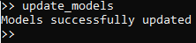
In order to see this, we’ll first need to update the statistical models for all of the terms [primitive and non-primitive] currently known to the interpreter. We may do so by invoking the update_models command, like so:

Depending on the nature and number of the terms that were evaluated prior to using the update_models command, this operation may take a little while to complete, but in our particular case, we can expect this particular usage to finish almost instantly. With models updated based on all of the terms we have previously evaluated, which included +1 on vectors #0[1.0] through #0[10.0], at integer increments, we may now check the content of the learned model by using the simulate command on expressions that we wish to see a modeled response for.

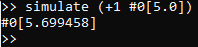
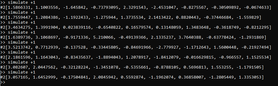
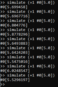
While the actual result of eval (+1 #0[5.0]) is #0[6.0], we can see that the simulated result is not terribly far off from what we would expect. However, only showing one result of this particular command-line is bound to be somewhat misleading, since actually, simulate samples from a distribution over models, representing (in a Bayesian sense) the current beliefs about what models are most likely to match the already-observed evaluation results. In particular, if we invoke the above command multiple times, we will see a range of outcomes, much like the following trace:

Embeddings

Being able to simulate expressions with vector outputs without actually evaluating them is somewhat neat, but what about expressions that have functions as outputs? Well, simulate works in this setting as well, as we can see from the following example of invoking it on the function +1.

As we can see, the result looks like some kind of vector inhabiting the type #2, but #2 is a function type! The reason for this is that actually, the printed vector corresponds to a particular embedding sample for a function of the type #2. An embedding sample may be thought of as corresponding to a particular modeled function that FETISH believes that a model could actually represent. In the context of FETISH, a (generalized) embedding refers to the distribution that a model of a term defines over embedding samples for that term.

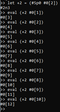
In light of the above description, and much like the previous case where we had a vector output, repeated simulation of +1 yields different embedding samples every time, which are all drawn from the same model:

As we can see, there may be significant variation in the sampled embeddings between each call to simulate in this setting where we have only evaluated our terms on very few data-points. In general, as we evaluate more terms [and subsequently issue an update_models command], the covariance in repeated embedding samples will tend to shrink, until eventually we obtain some kind of limiting distribution over embedding samples. If the underlying function term has deterministic behavior, then we can expect convergence toward one particular embedding sample in the limit.

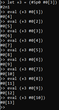
However, we can also say more about embedding samples when we consider multiple distinct terms (with multiple, different corresponding models). For an example, suppose that we define non-primitive terms +2 and +3 analogously to +1, and evaluate them all on the same data-points, like so:

Then, while we could update_models and then draw a bunch of samples from each of +1, +2, and +3 looking for patterns, we could instead extract the mean embedding sample for each using the get_mean command, like so:

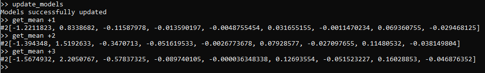
From these outputs, we can see that there’s a clear trend going from +1 to +3, and that, for instance, the mean embedding sample for +2 is closer to +1’s than +3’s is. This property, where function terms with greater similarity in behavior tend to have closer sampled embeddings, is the reason why we bother calling them embeddings in the first place, in analogy to e.g: word embeddings in natural language processing.

Epilogue

The above tutorial was only a small taste of what you can do with FETISH – more in-depth information may be found on this other post of mine. Overall, the hope of this research project is that by systematically deriving embeddings for terms in a small functional language, it will eventually possible to leverage machine learning algorithms to automatically construct programs that exhibit desired behavior. While there are some definite obstacles along the way (e-mail the author at ajg137@case.edu if curious, or wait for more articles to come), incremental progress is much better than no progress on such an important pursuit.